CMUQ 15-121 Searching & Sorting

1. Introduction
2. Searching
- 2.1. Linear Search
- 2.2. Binary Search
3. Sorting Algorithms
4. Definition: Stable Sorts
5. Sorting Summary Table

1. Introduction

In this set of notes we’re going to look in a bit more detail at two important functions that frequently performed on data structures: Searching and Sorting.

2. Searching

Searching is the process of looking through the data contained in a data structure and determining if a specific value is present. (And potentially returning it.) The contains methods of the ArrayList, for example, is a method that searches the list for a given value and returns true of false.

2.1. Linear Search

The most basic search algorithm is a linear search. This is just a fancy name for “start at the first element and go through the list until you find what you are looking for.” It is the simplest search. Here is a simple implementation for an array:

public static int linearSearch(int[] a, int value) {
    int n = a.length;
    for (int i = 0; i < n; i++) {
        if (a[i] == value)
            return i;
    }
    return -1;
}

If you look carefully at it, you’ll realize that the efficiency is \(O(N)\). Is it possible to do better than this, though?

2.2. Binary Search

Binary search is a searching algorithm that is faster than \(O(N)\). It has a catch, though: It requires the array you are searching to already be sorted. If you have a sorted array, then you can search it as follows:

Imagine you are searching for element v.
Start at the middle of the array. Is v smaller or larger than the middle element? If smaller, then do the algorithm again on the left half of the array. If larger, then do the algorithm again on the right half of the array.

Basically, with every step, we cut the number of elements we are searching for in half. Here is a simple implementation:

public static int binarySearch(int[] a, int value) {
    int lowIndex = 0;
    int highIndex = a.length - 1;
    while (lowIndex <= highIndex) {
        int midIndex = (lowIndex + highIndex) / 2;
        if (value < a[midIndex])
            highIndex = midIndex - 1;
        else if (value > a[midIndex])
            lowIndex = midIndex + 1;
        else // found it!
            return midIndex;
    }
    return -1; // The value doesn't exist
}

The efficiency of this is more complicated than the things we’ve been analyzing so far. We aren’t doing \(N\) work in the worst case, because even in the worst case we are cutting the array in half each step. When an algorithm cuts the data in half at each step, that efficiency is logarithmic. In this case, \(O(\textrm{log}_2\textrm{ } N)\). In efficiency, we frequently drop the base 2 from logarithmic efficiency, so we can just write this as \(O(\textrm{log } N)\). This is significantly better than an \(O(N)\) algorithm.

3. Sorting Algorithms

Binary search is great, but it requires your array be already sorted. So, how do we sort an array? This is a big question, and there has been a lot of work in the field of Computer Science to figure out the best ways to sort. Let’s go over some common algorithms along with their efficiencies.

Please note that there is an amazing website called visualgo that has nice illustrations of most of these algorithms. As you go through these notes, visit it to watch the algorithms in action and improve your understanding. The notes here are not sufficient to properly understand the algorithms, you should use the visualization as well.

3.1. Bubble Sort

Bubble sort is an easy algorithm based on going through the array and swapping pairs of numbers. The algorithm works as follows:

Algorithm

Starting with the first element, compare it to the second element. If they are out of order, swap them.
Compare the 2nd and 3rd element in the same way. Then the 3rd and 4th, etc. (So, go through the array once doing pair-wise swaps.)
Repeat this N times, where N is the number of elements in the array.

There are a few observations you can make that can speed this up a bit:

After the first pass, the largest element is at the end. After the second pass, the second largest element is second to the end, etc. (This means each pass you make doesn’t actually need to go through the entire array, later passes can stop earlier.)
If you make a pass and don’t perform any swaps, then the array is sorted.

Sample Implementation

public void bubbleSort(int[] a) {
    int n = a.length;
    boolean didSwap = true;
    
    // Keep going until we didn't do any swaps during a pass
    while (didSwap) {
        didSwap = false;
        // Make a pass, swapping pairs if needed.
        for (int i = 0; i < n - 1; i++) {
            if (a[i] < a[i + 1]) {
                didSwap = true;
                swap(a, i, i + 1);
            }
        }
        // The previous loop puts the largest value at the end,
        // so we don't need to check that one again.
        n--;
    }
}

Efficiency

In the worst case (even doing the optimizations mentioned above) the first pass does (N-1) compares and swaps. The second pass does (N-2) compares and swaps, etc. This happens N times. This makes the efficiency \(O(N^2)\).

3.2. Insertion Sort

Insertion sort is the type of sorting most people do if you give them a set of 7 playing cards, out of order, and ask them to sort them in their hand.

Algorithm

In each iteration, i, take the element in the i^th position, compare it to the one before until you find the place where it belongs. (In other words, while it is less than the one behind it, keep moving it backwards.)

Sample Implementation

public static void insertionSort(int[] a) {
    int n = a.length;
    for (int i = 0; i < n; i++) {
        int index = i;
        int valueToInsert = a[index];
        while (index > 0 && valueToInsert < a[index - 1]) {
            a[index] = a[index - 1];
            index--;
        }
        a[index] = valueToInsert;
    }
}

Efficiency

The overall algorithm “inserts” all N items individually, and each insertion takes N compares in the worst case. This makes the efficiency \(O(N^2)\). However, in practice, it is typically faster than bubble sort despite having the same big-o efficiency.

3.3. Selection Sort

Selection sort if based on the idea of “selecting” the elements in sorted order. You search the array for the smallest element and move it to the front. Then, you find the next smallest element, and put it next. Etc.

Algorithm

In each iteration, i, selection the i^th smallest element and store it in the i^th position. After completing N iterations, the array is sorted.

Sample Implementation

public static void selectionSort(int[] a) {
    int n = a.length;
    for (int i = 0; i < n - 1; i++) {
        int indexOfSmallest = i;
        for (int j = i + 1; j < n; j++)
            if (a[j] < a[indexOfSmallest])
                indexOfSmallest = j;
        swap(a, i, indexOfSmallest);
    }
}

Efficiency

There are N iterations of the algorithm, and each iteration needs to find the smallest element. Finding the smallest element is \(O(N)\), and doing an \(O(N)\) operating N times results in an effiency of \(O(N^2)\).

3.4. Merge Sort

Merge sort is a recursive algorithm that involves splitting and merging the array.

Algorithm

The algorithm works as follows:

Divide the array in half.
Recursively sort both halves.
Merge the halves back together.

Sample Implementation

public static void mergeSort(int[] a) {
    if (a.length > 1) {
        int mid = a.length / 2; // first index of right half
        int[] left = new int[mid];
        for (int i = 0; i < left.length; i++) // create left subarry
            left[i] = a[i];
        int[] right = new int[a.length - mid];
        for (int i = 0; i < right.length; i++) // create right subarray
            right[i] = a[mid + i];
        mergeSort(left); // recursively sort the left half
        mergeSort(right); // recursively sort the right half
        merge(left, right, a); // merge the left and right parts back into a whole
    }
}

public static void merge(int[] left, int[] right, int[] arr) {
    int leftIndex = 0;
    int rightIndex = 0;
    for (int i = 0; i < arr.length; i++) {
        if (rightIndex == right.length || (leftIndex < left.length && left[leftIndex] < right[rightIndex])) {
            arr[i] = left[leftIndex];
            leftIndex++;
        } else {
            arr[i] = right[rightIndex];
            rightIndex++;
        }
    }
}

Efficiency

The process of merging two sorted lists together is \(O(N)\). Merge sort, effectively, does this \(O(\textrm{log } N )\) times. (Because it splits the list in half at every step.) So, that makes the overall efficiency \(O(N\textrm{ log } N )\).

For a more detailed understanding of where the \(O(\textrm{log } N )\) comes from, check out this detailed explanation from Khan Academy.

diagram
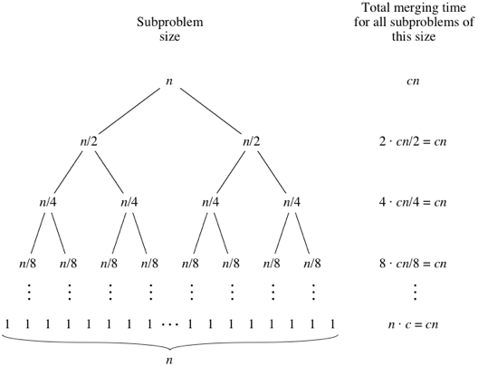
^{Image license: CC-BY-NC-SA. Courtesy of [Khan Academy]}

3.5. Quick Sort

Quick sort is an interesting algorithm because while its worst case is technically \(O(N^2)\), in practice it is almost always \(O(N\textrm{ log } N )\).

Quick sort is a recursive algorithm based around the idea of choosing a pivot item and sorting around it.

Algorithm

“Randomly” choose an element from the array as your pivot.
Partition the array around your pivot, making sure that items less than the pivot are to the left of it and all items greater than or equal to the pivot are to the right of it.
Recursively sort both parts.

Sample Implementation

public static void quickSort(int[] a) {
    quickSort(a, 0, a.length - 1);
}

public static void quickSort(int[] a, int low, int high) {
    if (low < high) {
        int pivotIndex = partition(a, low, high); // value at pivotIndex will be in correct spot
        quickSort(a, low, pivotIndex - 1); // recursively sort the items to the left (< pivot)
        quickSort(a, pivotIndex + 1, high); // recursively sort the items to the right (>= pivot)
    }
}

public int partition(int[] arr, int low, int high) {
    int pivot = arr[low]; // select the first value as the pivot value (there are better ways to do this!)
    int boundaryIndex = low + 1; // the index of the first place (left-most) to put a value < pivot
    for (int i = low; i < high; i++) {
        if (arr[i] < pivot) {
            if (i != boundaryIndex) { // if it is ==, no swap needed since it's on correct side of partition
                swap(arr, i, boundaryIndex);
            }
            boundaryIndex++; // must always bump boundary if a smaller element found at arr[i]
        }
    }
    /*
     * boundaryIndex is the first (left-most) index of values >= pivot, because all
     * elements to the left of boundaryIndex are < pivot so we'll swap the pivot (at
     * index high) with the value at boundaryIndex -1, so pivot is placed correctly
     */
    swap(arr, low, boundaryIndex - 1);
    return boundaryIndex - 1;
}

Efficiency

Analyzing the efficiency here is somewhat complicated by the choice of pivot. If the pivot is perfectly chosen each time, then the array is effectively split in half at each step. That would make the efficiency \(O(N\textrm{ log } N )\) for the same reason that merge sort is. However, in the worst case the pivot isn’t in the middle, instead it is at one of the ends. That would make the efficiency \(O(N^2)\).

So, which is it? Technically, the worst case complexity is \(O(N^2)\). However, in practice with a randomly chosen pivot each time, it is usually \(O(N\textrm{ log } N )\). It is also usually faster than merge sort, because the partitioning process is faster than merging.

4. Definition: Stable Sorts

A stable sort is one where, after sorting, the relative position of equal elements remains the same. Why is this useful? Let’s imagine you are sorting students and you want a list of students sorted by gender, but within gender you want them sorted by name. If you are using a stable sort, then you first sort the entire list by name and then sort the entire list by gender. The final list will have the ordering you want.

Bubble, insertion and merge sort are stable sorts. Selection and quick sort are not stable sorts.

Potential quiz/exam questions for you to think through:

Why is selection sort not stable?
Why is quick sort not stable?

5. Sorting Summary Table

Sort	Best Case	Average Case	Worst Case	Stable?
Bubble	\(O(N)\)	\(O(N^2)\)	\(O(N^2 )\)	Y
Insertion	\(O(N)\)	\(O(N^2 )\)	\(O(N^2 )\)	Y
Selection	\(O(N^2 )\)	\(O(N^2 )\)	\(O(N^2 )\)	N
Merge	\(O(N\textrm{ log } N)\)	\(O(N\textrm{ log } N )\)	\(O(N\textrm{ log } N )\)	Y
Quick	\(O(N\textrm{ log } N )\)	\(O(N\textrm{ log } N )\)	\(O(N^2 )\) (but see note above)	N