CMUQ 15-121 Priority Queues and Heaps

• 1. Introduction
• 2. Priority Queue
  • 2.1. PQ with an Array
  • 2.2. PQ with a Linked List
  • 2.3. PQ with a Binary Search Tree
  • 2.4. PQ Efficiency Summary Table
• 3. Binary Heap
  • 3.1. Operations
    • 3.1.1. Add
    • 3.1.2. Peek Max
    • 3.1.3. Remove Max
  • 3.2. New Efficiency Summary Table
  • 3.3. Array Implementation
  • 3.4. Heap Sort

1. Introduction

In this set of notes we’ll talk about a new abstract data type, the priority queue. Then we’ll evaluate the efficiency of implementing it using a variety of the data structures we’ve studied so far. Finally, we’ll introduce a new data structure, the binary heap, that can be used to very efficiently implement a priority queue.

2. Priority Queue

A priority queue is similar to a regular queue, but each item in the queue has an additional piece of information: Priority. When you remove from a priority queue, you remove the item with the highest priority. Here are some sample operations that a priority queue might have:

• add(DataType item, int pri) // Add an item to the queue who has priority pri
• DataType peekMax() // Peek at the item in the queue with the highest priority
• DataType removeMax() // Remove and return the item in the queue with the highest priority

There are a number of real-world applications of priority queues. They are part of most operating systems (programs are chosen to run based on their priority). Many network routers also use a priority queue to determine which packet to send next. (High priority traffic goes first.)

Let’s evaluate different ways we could implement a priority queue using our three main data structures so far: Array (or ArrayList), LinkedList, or a binary search tree.

2.1. PQ with an Array

If we implement the PQ with an array, there are two main approaches: An unordered array and a sorted array.

If we use an unordered array then add will be simply putting another item onto the end of the array, which is \(O(1)\) assuming the array is large enough. peekMax would require linear searching the entire array for the max value, which is \(O(N)\). removeMax would requiring linear searching the entire array, finding the item, removing it, and shifting all the entries after it in order to remove the hole in the array. This is also \(O(N)\).

If we use a sorted array then add will need to search for the correct location to place the new item (\(O(\textrm{log }N)\) if we do a binary search on the sorted data) and then shift down all the items that follow that space (\(O(N)\)) and adding the item. This makes add \(O(N)\) overall. peekMax would require simply returning the last item in the array, which is \(O(1)\). removeMax would require removing the last item and returning it, which would also be \(O(1)\).

2.2. PQ with a Linked List

With a linked list we have the same basic approaches as the array: unordered and sorted. Let’s look at both.

If we use an unordered linked list then add will simply be adding to the head of the list, which is \(O(1)\). peekMax would require a full search of the list, which is \(O(N)\). removeMax would effectively be the same as peekMax.

If we use a sorted linked list then add requires a full search in order to figure out where to put the new item, which is \(O(N)\). Assuming we store the nodes so that the highest priority item is the head of the list, then peekMax and removeMax become \(O(1)\) because the highest priority item is simply at the head of the list.

2.3. PQ with a Binary Search Tree

If we implement a PQ using a BST, then we would use the priority as the key to sort by.

Assuming the tree stays reasonably balanced (which might be a dangerous assumption), then add would be \(O(\textrm{log }N)\) to find the correct location in the tree and add the new node. peekMax and removeMax would simply require searching in the tree, which would also be \(O(\textrm{log }N)\).

2.4. PQ Efficiency Summary Table

Here is a summary of the efficiency of a priority queue depending on the data structure we use to implement it:

^* The BST efficiencies assume a balanced tree, which is not guaranteed. Actual efficiencies may be worse than stated.

Can we do better than this? The answer, of course, is yes. We just need a new type of data structure.

3. Binary Heap

A binary heap is a type of binary tree (but not a binary search tree) that has the following properties:

1. Shape: It is a complete tree. (Remember that a complete binary tree is one where every level except the last one is completely filled, and the last level has all leaves as far left as possible.)
2. Order (heap): The parent of a node is \(\ge\) all of its children (for a max heap) or \(\le\) all of its children (for a min heap).

Throughout these notes I will be using examples of a max heap.

Here is a sample:

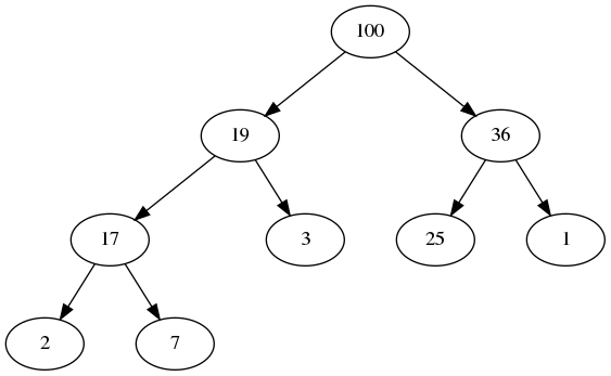
Notice that this is not a BST. Left and right ordering is not relevant. Instead, it maintains the shape and heap properties we just talked about. Pause for a moment here to study the tree and make sure you understand both properties properly.

3.1. Operations

If we were to build a priority queue using a binary heap, how would the operations work and what would be the efficiency?

3.1.1. Add

If we want to add to a binary heap, we need to ensure that our two properties are maintained after the new node is added. Let’s consider the binary heap above and say that we want to add 33 to it. In order to ensure that the tree remains a complete tree, we must add the new node at the last level, as far left as possible. So, if we add 33 there, we end up with:

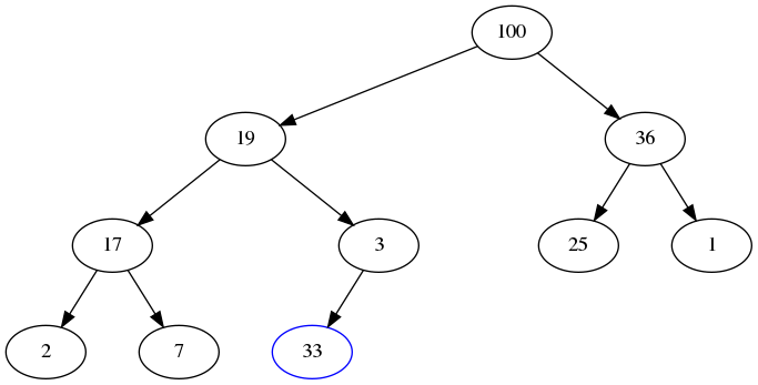
We still have a complete tree, which is good, but now the tree violates the heap property. (33 is below 3, and that should never happen.) In order to fix this, we will heapify up by continually swapping 33 with its parent until it is in the correct location:

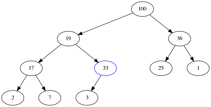
1. First, we notice that 33 is greater than its parent 3, so we swap them:
2. Then, we notice that 33 is larger than its new parent, 19, so we swap them:
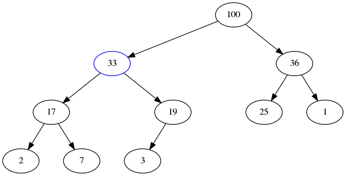
3. Now we notice that 33 is smaller than its parent, so we stop.

The process of adding the node to the bottom of the tree is \(O(1)\). The process of heapifying up the tree is \(O(\textrm{log } N)\). An \(O(1)\) operation followed by a \(O(\textrm{log } N)\) operation is just \(O(\textrm{log } N)\). This is guaranteed worst-case efficiency; unlike the BST, where we assume a balanced tree, a binary heap guarantees a complete tree.

3.1.2. Peek Max

If we want to quickly peek and see the largest node in the heap, that is easy. Just return a pointer to the root. This is \(O(1)\).

3.1.3. Remove Max

Removing the maximum item from the heap is a bit more complicated that just peeking. Finding the max item is \(O(1)\), but actually removing it requires additional effort.

Imagine we want to remove the max item from the last heap picture given above. There are two conflicting things we need to manage at the same time:

1. We want 100 to be gone from the heap.
2. The node that actually disappears needs to be the node storing 3. (Because after the remove the tree has to be complete.)

Let’s handle this the laziest way possible, and hopefully we can do a swapping trick later to fix up any problems. Let’s just remove node 3, and replace 100 with 3:

The good thing about this is that it is still a complete tree. The bad thing is that it doesn’t satisfy the heap property anymore. To fix the heap property, we will heapify down by continually swapping 3 with its largest child that is bigger than 3.

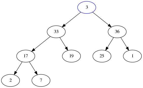
1. Swap with 36. (Because 36 is the largest child and is bigger than 3.):
   
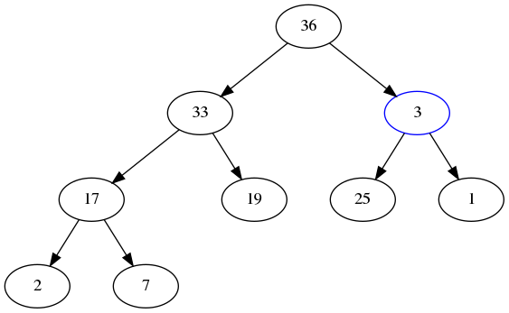
2. Swap with 25. (Because 25 is the largest child and is bigger than 3.):
   
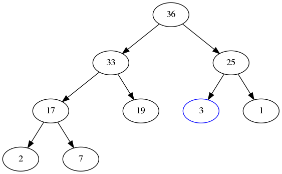
3. Now we notice that 3 is not smaller than its children. (Plus, it has not children.) So we stop. The heap is valid again.

This entire process is \(O(\textrm{ log } N)\), much the same reason that add is.

3.2. New Efficiency Summary Table

Here is a completed efficiency summary table for a priority queue, now including the binary heap:

^* The BST efficiencies assume a balanced tree, which is not guaranteed. Actual efficiencies may be worse than stated.

In general, a binary heap is going to be the best data structure for a priority queue. (Although it may vary somewhat depending on the details of implementation.)

3.3. Array Implementation

While we illustrated the binary heap using a traditional tree diagram, in practice it is perfectly suited for implementation using the array representation of binary trees presented in the previous notes. While doing an add it is easy to find the next empty location in the complete tree (it is the next empty location in the array). Likewise, when doing a remove, finding the last node in the tree (the last used spot in the array) and swapping it into the root is also easy. Finally, the heapify procedure is also straight-forward.

You should practice the binary heap operations on a binary heap stored in an array. That sort of thing seems like a really nice quiz or exam question…

3.4. Heap Sort

One final note about binary heaps: You can also use the concepts from a binary heap for sorting. We call that sorting algorithm heap sort. The basic concept is that you build a heap using the unsorted values and then continually remove the largest item from the heap, creating the sorted order. The algorithm is \(O(N\textrm{ log } N)\), but it is not a stable sort.

For more details, checkout the Wikipedia article on heap sort.